When “one size fits all” fails: PostGIS bounding boxes for maps

As a mapping company, we curate and visualize all sorts of data for our users. Part of delivering this experience is making sure that it’s easy to interact with data layers (e.g. emphasizing fast tile delivery, letting you filter legend items and/or click geometric attributes for additional detail). “Making sure it’s easy,” is not an easy thing to do, however.

The world, and the data we use to represent it, is complicated and varied. Great maps are often the result of a series of subjective decisions on what to do with that data; they are purpose-built to communicate ideas and information more effectively. At Felt, we are constantly exploring how to deliver the "right" experience at scale. But what if there are different "right" ways, and no one-size fits all solution? For the engineers at Felt, this means plunging into the messy world of reality and embracing heuristics over universal formulas.

Zoom to fit & PostGIS

Being able to see the extent of a single data layer may sound like a pretty straight-forward, one size could possibly fit all problem–right? Wrong. We found that determining the right extent for a data layer requires a heuristic approach. First, some context about the Zoom to fit feature.

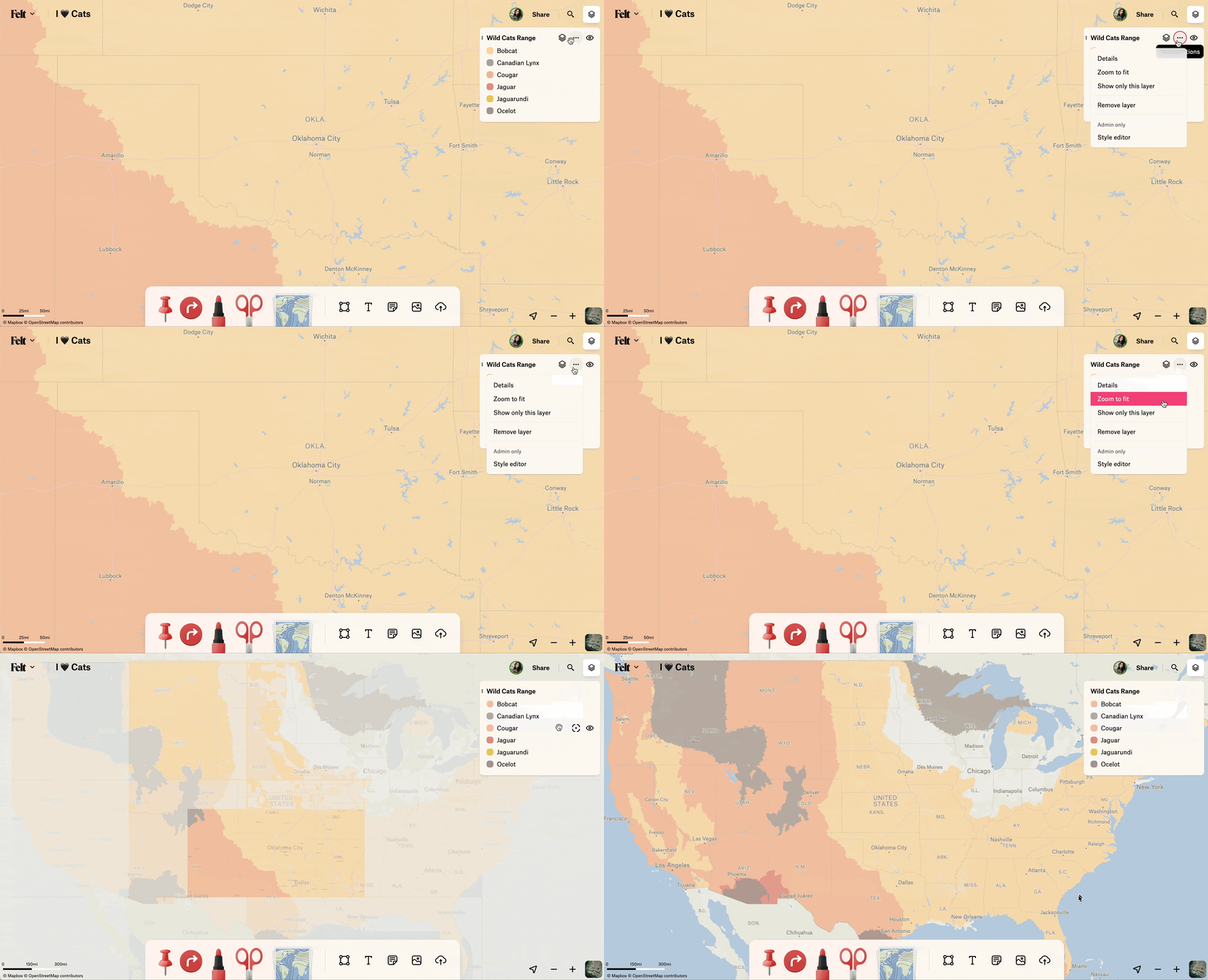
When we decided to implement the feature, one of the first decisions was which part of the stack is responsible for the calculation, the frontend or the backend. If we were working on small datasets with relatively few, clustered points, it would be tempting to push the responsibility to the frontend. However our data layers are large, often consisting of thousands of geometric features that can span the whole globe. Additionally, the frontend is receiving tiles piecemeal so it won’t always immediately have the full picture of the data. To avoid burdening the frontend with a slow and complex calculation, we decided to take advantage of PostGIS functionality to calculate bounding boxes during upload processing and deliver these bounds to the frontend as geojson polygons along with other layer metadata. During the processing stage, we import our layers into PostGIS, which creates tables consisting of rows of various geometric elements. PostGIS gives users a few different query options to calculate a bounding box for different geometries or sets of geometries. In PostGIS terms, this is often referred to as the extent. Let’s take a look at a few different extension functions that let us calculate the extent of our data.

PostGIS Extent Calculations

PostGIS gives us some different options for calculating bounding boxes for our data:

ST_Extent: “An aggregate function that returns a box2d bounding box that bounds a set of geometries.”
ST_EstimatedExtent: “Returns the estimated extent of a spatial table as a box2d. The current schema is used if not specified. The estimated extent is taken from the geometry column's statistics.”
ST_3DExtent: “An aggregate function that returns a box3d (includes Z ordinate) bounding box that bounds a set of geometries.”
ST_Envelope: “Returns the double-precision (float8) minimum bounding box for the supplied geometry, as a geometry.” Crucially, this is only used for a single geometry, not for a whole table.

Given that we’re operating on the 2D plane and need to evaluate multiple geometries, we can disregard <p-inline>ST_3DExtent<p-inline> and <p-inline>ST_Envelope<p-inline>. The question becomes whether to use <p-inline>ST_Extent<p-inline> or <p-inline>ST_EstimatedExtent<p-inline>. Both can be useful in different situations. <p-inline>ST_Extent<p-inline> does the heavy lifting of calculating an accurate bounding box, but for large tables, this can come at a cost. <p-inline>ST_EstimatedExtent<p-inline>, on the other hand, is basically a “free” calculation. Rather than actually calculating the bounding_box for every row, <p-inline>ST_EstimatedExtent<p-inline> takes advantage of Postgres autovacuuming to regularly sample the table and store statistics on it. When you make a request <p-inline>ST_EstimatedExtent<p-inline> will give you a pre-calculated extent that is roughly 95% of the actual <p-inline>ST_Extent<p-inline> calculation.

But just how much faster is it? I wanted to get a better idea and so I ran a test on one of our larger data layers– a table with 242,747 rows of multipolygon geometries. In the table below, you can see the average execution time for 50 runs, as well as the resulting bounding box.

As you can see, both functions output very similar polygon bounding boxes. While <p-inline>ST_EstimatedExtent<p-inline> is much faster, <p-inline>ST_Extent’s<p-inline> execution time makes it more than suitable, especially if these calculations are being processed during some sort of background task. One of the reasons for choosing <p-inline>ST_Extent<p-inline>, as mentioned above, is accuracy. There are, however, reasons to use <p-inline>ST_Extent<p-inline> that go beyond accuracy and speed.

Shifting geometries for better bounding boxes

Of course, things aren’t necessarily so simple. Take a look at this bounding box for US Census Block Groups. Everything looks good, but when we go to graph the calculated bounding box, it spans several continents! Regardless of whether you use <p-inline>ST_EstimatedExtent<p-inline> or <p-inline>ST_Extent<p-inline> you will get something that looks roughly like below.

This isn’t the optimal box for a US Census layer.

So what happened, and how can we fix it? The answer here is that the dataset includes the U.S. territory of Guam, which causes the data to stretch the whole world. We typically project the world as being a surface between 180°W (-180° E) and 180°E, for a total of 360° of longitude. Guam is ~144° E (Hagåtña, the capital of Guam, is at 144° 45′ 0″ E).

The line through our bounding box is the 180th meridian, or antimeridian, which functions as a start and end point for our extent calculation.

While the bounding box is technically correct, we can “wrap” the longitudes to get a tighter bounding box using the ST_WrapX function. In essence we are recentering our data such that the “antimeridian” is not the start/end point. Instead we pick a longitude that is more favorable.

This, however, means that we cannot use <p-inline>ST_EstimatedExtent<p-inline>. We can’t simply shift the coordinates of a calculated bounding box, but instead, we need to “correct” every geometry and then calculate the extent. Since <p-inline>ST_EstimatedExtent<p-inline> relies purely on table statistics, it is not an option. We must shift the geometries and then use<p-inline> ST_Extent<p-inline> to get the bounding box for these points.

Let’s recalculate. First, we pick a longitude which will provide a more favorable projection. The <p-inline>ST_WrapX<p-inline> function “splits the input geometries and then moves every resulting component falling on the right (for negative 'move') or on the left (for positive 'move') of given 'wrap' line in the direction specified by the 'move' parameter, finally re-unioning the pieces together.”

What we are trying to do is find a longitude that doesn’t have geometries clustered tightly to both sides of the line. Our data points should all fall to the right or left of the given line. Given that Guam is ~144° E, let’s pick the 135th meridian east and shift our data. Every geometry greater than 135° E right of the line below will be shifted -360°.

We run the following <p-inline>SELECT ST_AsGeoJSON(ST_Extent(ST_WrapX(geom, 135, -360))) as extent FROM us_census_blocks<p-inline>

At 3.26 seconds of execution time, we get the above result. Even though we take a bit of a hit to shift our geometries, the resulting box is much tighter! Getting an optimal bounding box for display isn’t as simple as running the above formula on any given set of geometries. The formula that works above can suffer with a different set of data. For example, look at what happens if we generate a bounding box for the riverways of Asia, which has points clustered on either side of this line.

<p-inline>SELECT ST_AsGeoJSON(ST_Extent(ST_WrapX(geom, 135, -360))) as extent FROM riverways_asia<p-inline>;

Now compare this to the output when we don’t shift our data.

<p-inline>SELECT ST_AsGeoJSON(ST_Extent(geom)) as extent FROM riverways_asia<p-inline>;

There is an important lesson here that we should remember whenever we’re working with geospatial data. Making an arbitrary decision about where data “starts” and “ends” when projecting a sphere into two-dimensions is ultimately a subjective cartographic choice that is relative not only to each dataset, but what we’re trying to learn from it. In this case, we could probably develop a pretty good heuristic for a given dataset by sampling random points, but there’s not a one-size-fits-all solution.

As you can see, calculating bounding boxes isn’t a trivial matter, but PostGIS gives us some great tools for this work. We’re lucky to be a part of a vibrant open source community that has developed some great tools for working with geospatial data. If you’re looking for a chance to play with some of these technologies, and build the next generation of maps, we’re hiring!

Zoom to fit & PostGIS

PostGIS Extent Calculations

Shifting geometries for better bounding boxes

Cartography Tips for Designing Web Maps

Search, filter, select — data discovery done right

Getting the most out of Felt’s new Workspaces

Teaching Spatial Analysis with Felt

Powerful new admin tools and a streamlined billing experience

Three key UI upgrades in Felt 2.0