Understanding geographically weighted regression and how it works

‍

Cities, farms, and ecosystems don’t behave the same way across every square inch of land. Housing prices rise on one block and stall on the next. Crop yield shifts across a single field. Canopy cover thickens and thins in a matter of meters. These variations matter — but they’re hard to spot when tools assume the whole model plays by the same rules.

To better understand what’s happening on the ground, analysts need regression models that account for local variation rather than lumping all the statistics together. Geographically weighted regression (GWR) provides that framework. It shows how relationships between variables change as you move across a landscape, giving more weight to nearby data points. That makes it possible to see, for example, how green space impacts rent prices across different neighborhoods. 

In this article, we’ll break down the meaning of GWR, how it works, and share real-world examples of how teams use it to make sense of complex spatial patterns. 

What’s geographically weighted regression?

GWR is a statistical method that reveals how patterns and relationships shift across different spaces. This is different from traditional regression, also known as ordinary least squares (OLS), which assumes that the same relationship holds everywhere across a map. 

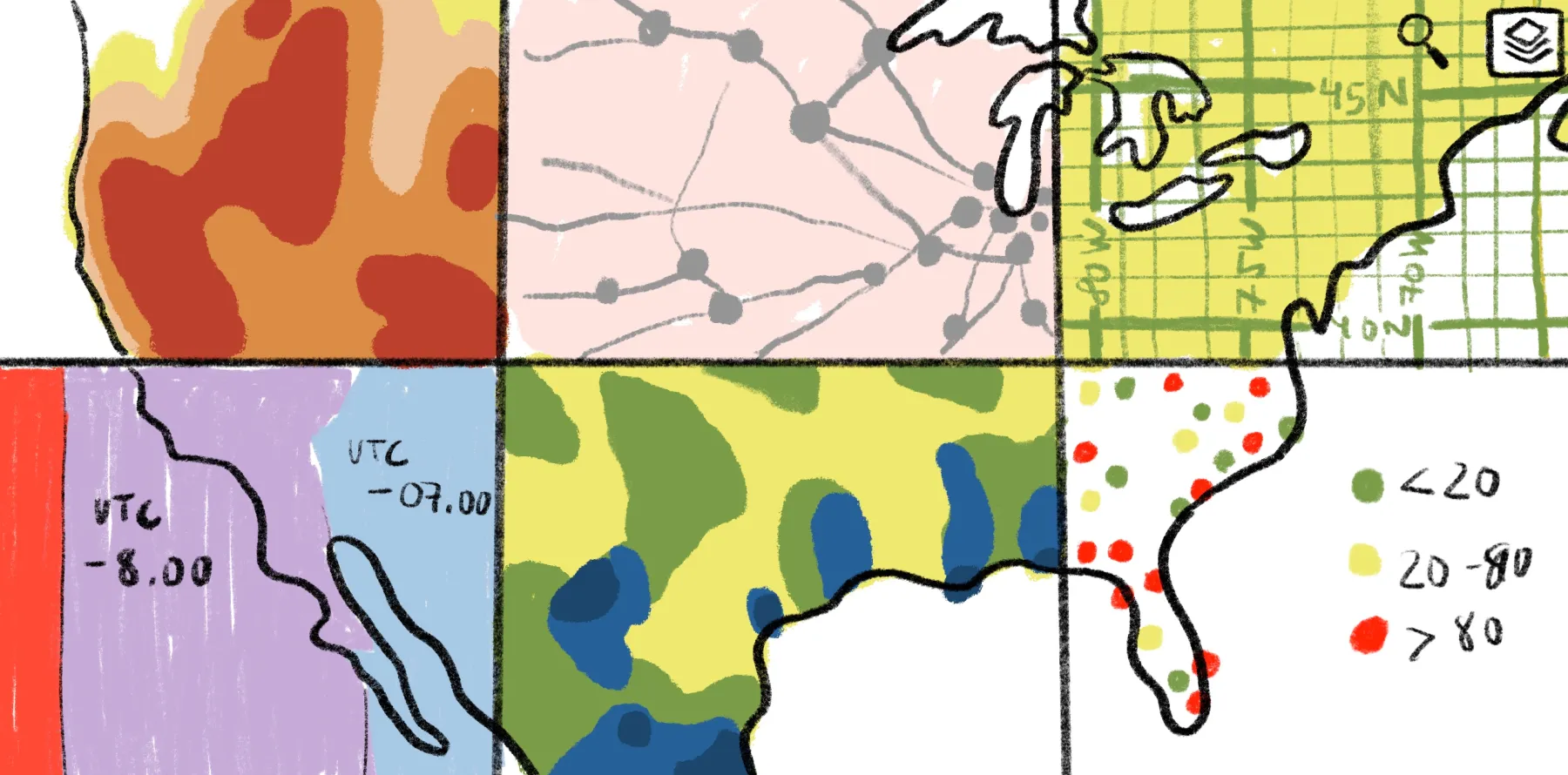
Imagine a city like Phoenix, Arizona, where extreme summer heat waves lead to sharp increases in heat-related illnesses. A traditional OLS regression map might show a citywide correlation between household income and heat-related illnesses. But since it applies a global equation to the entire map, it can’t reveal which neighborhoods are most at risk. 

GWR breaks the city map into smaller zones and weights nearby data points more heavily than ones farther away. The geographically weighted regression reveals exactly how and where income predicts higher instances of heat stroke and how those correlations vary geographically. 

What does weighted mean in GWR? 

In GWR, the model gives more influence to data points that are physically closer to one another. You start with a dependent variable — in this case, heat illness — and test out different explanatory variables, like household income. You could also choose to examine explanatory variables like asphalt coverage, population density, or demographics. 

By applying weighted regression, analysts uncover local correlation patterns. These statistics highlight where relationships strengthen or weaken.

Weighting GWR with the kernel function

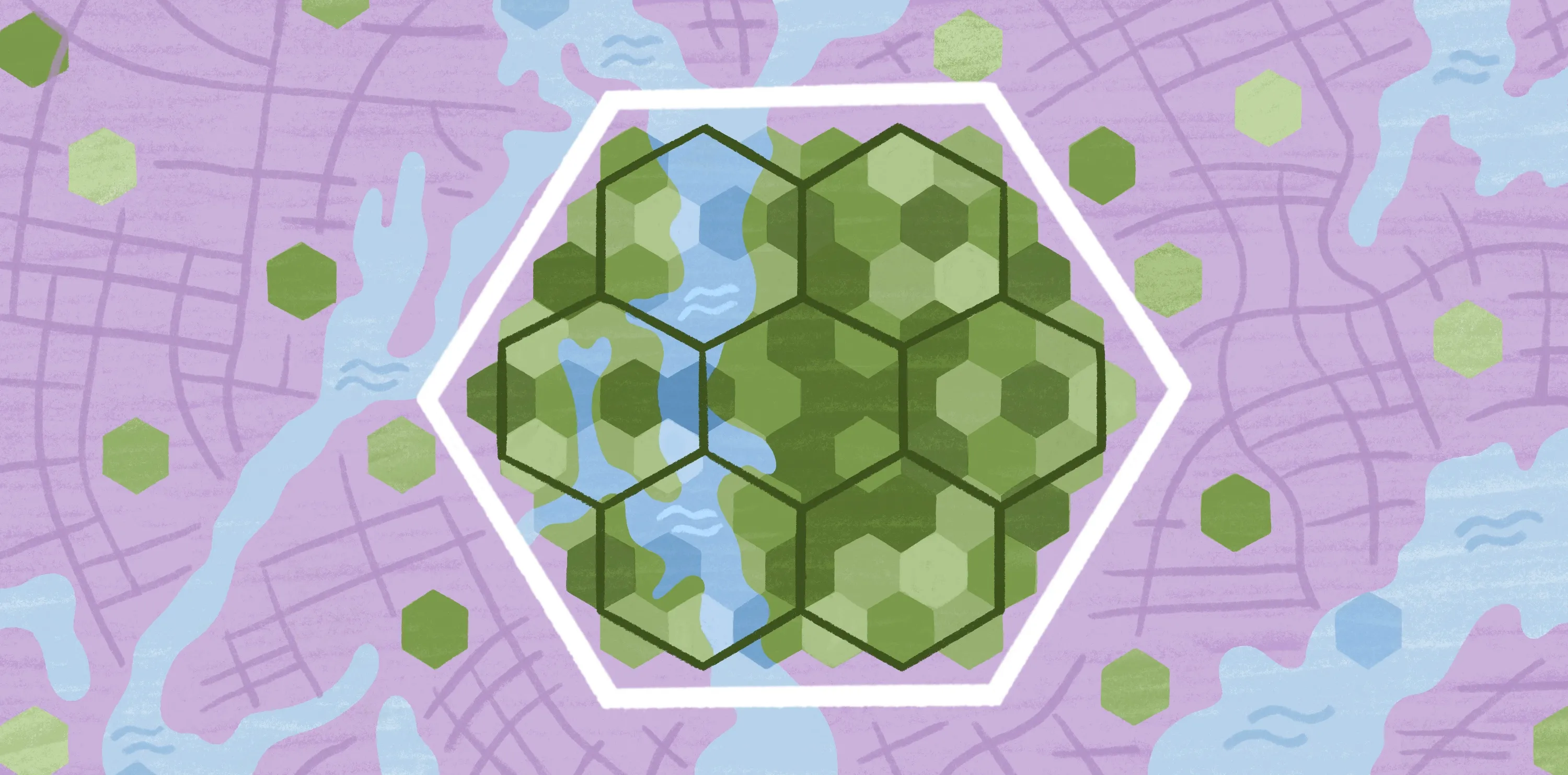
The kernel function is what controls the weighting in GWR. Each location receives its own regression model, and the kernel determines how much influence each data point has on that specific regression model. 

Closer data points matter more than distant ones, and the kernel defines how quickly that influence fades with distance. The fading influence is often called distance decay. The rate at which the distance decays is determined by the bandwidth. Small bandwidth keeps your spatial analysis extremely local, whereas a large bandwidth pulls spatial data from a larger section of the map. 

Analysts can choose from different types of kernels. The most common include: 

• Gaussian kernels: Weight decreases as distance increases, giving nearby variables the strongest influence over the local regression model. 
• Bisquare kernels: Weight decreases with distance and reaches zero once an explanatory variable moves beyond a specified bandwidth, keeping local models tightly focused. 

Why do kernel functions matter to spatial analysis? 

When you apply distance-based weights, GWR generates local estimates instead of a global pattern. Each location ends up with its own set of regression coefficients — statistics that describe how strongly each explanatory variable affects the dependent variable in a specific area. These geographically varying coefficients illustrate where relationships strengthen and weaken.

They also tend to expose residual patterns, which are the differences between actual and predicted values at each location. Clusters of residuals often signal errors like missing variables in the model. Making adjustments — such as adding explanatory variables or adjusting the bandwidth — improves correlation estimates and strengthens spatial interpretation. 

How geographically weighted regression works

Here’s a look at the workflow GWR follows and how each step produces regression coefficients that reflect geographical variation. 

1. Input your spatial data

GWR starts with a spatial dataset containing your dependent variable and the explanatory details you want to test. These numeric variables allow the model to calculate local estimates geographically. By preparing accurate inputs, analysts ensure regression coefficients reflect meaningful spatial variation across the study area. 

2. Apply local weighting

Choose your bandwidth and kernel function. These settings determine how strongly nearby data points influence each local regression. For highly local results — like mapping how tree cover affects temperatures on a block-by-block scale — you might choose a small bandwidth and bisquare kernel function to focus the local regression model tightly around each location. 

To explore broader spatial trends — like how soil health changes across a farm belt region — a large bandwidth and a Gaussian kernel function allows the model to draw from a wide area and more generalized patterns. 

3. Run multiple local regressions

With spatial data and local weighting in place, GWR fits a separate local regression model at every location in the dataset. Each site produces regression coefficients, reflecting how strongly each explanatory variable affects the dependent variable in that specific area. These outputs form coefficient surfaces — spatial layers that illustrate how each coefficient changes geographically. 

In the case of a block-by-block analysis, each block will have its own coefficient, revealing how the relationship varies from one to the next. 

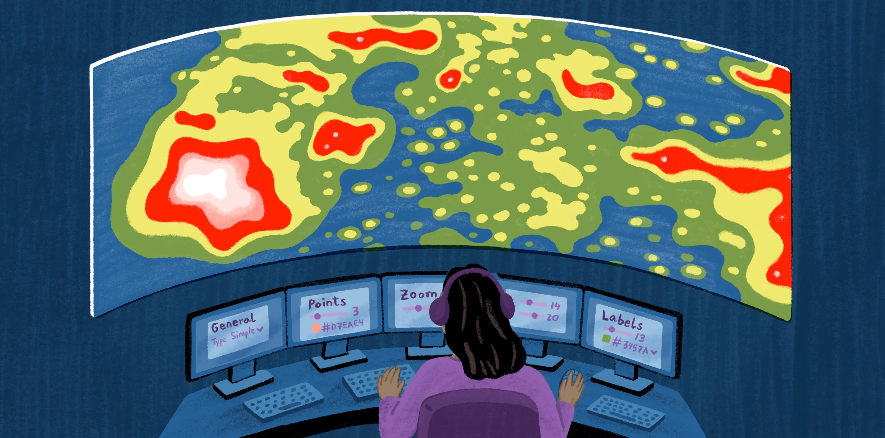
4. Visualize spatial variation

Analysts turn to GWR to produce a set of location-specific estimates. They then must visualize them using a GIS platform like Felt, which has data visualization tools to turn coefficient surfaces into readable, interactive maps. This allows you to compare how each explanatory variable influences the dependent variable across space. With Felt, you can toggle between variables and layer additional spatial data to see where relationships strengthen, weaken, or reverse. 

What’s GWR in practice? Here are some real-world applications

GWR helps reveal how a single variable can differ dramatically from a single city block, county, or region to the next. Decision-makers use GWR to calculate where and why variation occurs. Here’s a look at common real-life uses. 

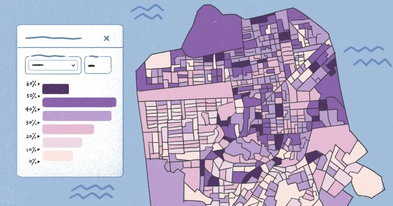
Urban planning

City planners use GWR to understand how public transportation, walkability, or household income influence property values across a city. Rather than examining a single citywide trend, a coefficient surface might show that transit access predicts home value strongly downtown but has little impact on the city’s far borders. Mapping out these shifting coefficients could highlight where planners can target transportation investments. 

Environmental management

Researchers turn to GWR to explore spatial patterns in pollution, vegetation, and soil composition. For example, regression analysis might be used to understand the impact of air pollution in industrial zones on respiratory illness or soil health in a specific region. Residual patterns highlight where models need refinement to calculate safe distances between housing, agriculture and high-exposure areas. 

Public education

GWR provides educators with spatial analysis showing how local policy influences student outcomes. For example, transit access may strongly impact attendance in one area, while food availability shapes grade point average in another. Mapping these shifts helps local governance determine resource allocation. 

Simplify complex spatial analysis with Felt AI

GWR uncovers rich spatial patterns. But those insights only become useful when they’re easy to see and share. Felt AI turns local regression outputs into clear, interactive maps so teams can understand complex spatial data with confidence. 

With Felt’s interactive platform, you can easily import datasets, visualize regression results, and collaborate on interpretations with shared maps and annotations. Try Felt today to turn advanced geospatial models into maps your whole team can use to drive stronger decision-making. 

FAQ

How does GWR differ from standard regression?

Standard regression applies one equation to the entire dataset. GWR builds several local regression models to observe how relationships change across space. 

What kind of data is required for GWR?

GWR requires a dependent variable, explanatory variables, and their corresponding numerical coordinates. Observations must have a location so the local regression model can calculate distance-based weights. 

Is GWR the same as weighted logistic regression?

GWR and weighted logistic regression both assign weight to certain datasets. However, weighted logistic regression is used to analyze data that is biased or skewed toward one group or condition. Weight is added to minority groups or conditions to balance it all out.